It could possibly be non-integrable, for example?My guess is that this works as long as the coeff b(x) is benign.
Or even ODE with discontinuous RHS
[$]\dot{x} = sgn (t)[$] for all values of [$]t[$].

Serving the Quantitative Finance Community

It could possibly be non-integrable, for example?My guess is that this works as long as the coeff b(x) is benign.
Back to this test case,Alan,
NY = 500 = NT using Roberts Weiss fdm (max err= 3,52e-5)
NY = NT = 1000, err = 1.1e-5
NY = NT = 2000, err = 3.21e-6
// copy from Excel not always works
X MOC exact solution X FDM solution
0 0.385821 0 0.385824
0.002 0.38582 0.002 0.385822
0.004 0.385818 0.004 0.385821
0.006 0.385816 0.006 0.385819
0.008 0.385814 0.008 0.385817
0.01 0.385812 0.01 0.385815
0.012 0.385811 0.012 0.385813
0.014 0.385809 0.014 0.385811
0.016 0.385807 0.016 0.385808
0.018 0.385805 0.018 0.385806
0.02 0.385803 0.02 0.385804
0.022 0.385802 0.022 0.385802
0.024 0.3858 0.024 0.3858
0.026 0.385798 0.026 0.385797
0.028 0.385796 0.028 0.385795
0.03 0.385794 0.03 0.385792
0.032 0.385792 0.032 0.38579
0.034 0.385791 0.034 0.385788
0.036 0.385789 0.036 0.385786
0.038 0.385787 0.038 0.385784
0.04 0.385785 0.04 0.385782
0.042 0.385783 0.042 0.385781
0.044 0.385781 0.044 0.385779
OK. Well at T=20 you are only examining the initial data from y=20/21 to y=1. So, next put a discontinuity halfway in-between at y=41/42. For example:
[$]f(y) = e^{-y} \times 1 \left(y > \frac{41}{42}\right) + 3 \times 1 \left(y \le \frac{41}{42}\right)[$],
where [$]1(condition)=1[$] if the condition is true and 0 otherwise.
Now your output (for your X=0 to 1) should start at 3 for about the first half and then jump to your previous results for the remainder of it. The exact [$]y[$]-jump point in the solution is where, at your T, [$]\xi = \frac{41}{42}[$] -- something like the solution to
(*) [$]\frac{20 - 19 y}{21 - 20 y} = \frac{41}{42}[$].
I really wish you hadn't switched from y to X, as it just makes it that much harder to discuss! Anyway, solve (*) and see if your solution jumps at that value of your X.
[$]u_t+u_y=0[$] .What's the pde you re looking at with these conditions?
Just one more thing before we jump headfirst into numerics:So
[$]u(y,t)= 1 [$] when [$]|y-t| \le 1/3[$]
[$]u(y,t)= 0 [$] when [$]|y-t| \gt 1/3[$].
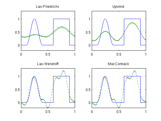
I have found a good test case from Matlab (squared cosine function and a double step function (my test only takes the more difficult latter) showing how FD methods behave. What we see here is Lax-Friedrichs is diffusive. The 2nd order methods preserve smooth profile but introduce spurious oscilllations around the 2 discontinuities. BTW the classic upwind scheme is less diffusive than LF.
When you solve numerically does the discontinuity disappear, e.g. spurious diffusion?

X MOC exact solution X Lax - Friedrichs
- 1 - 0.047012512 - 1 9.26536E-05
- 0.95 0.109823181 - 0.95 0.062928934
- 0.9 0.263954822 - 0.9 0.127034635
- 0.85 0.411587402 - 0.85 0.190821631
- 0.8 0.54908593 - 0.8 0.252637116
- 0.75 0.673064937 - 0.75 0.310813037
- 0.7 0.780471826 - 0.7 0.363718603
- 0.65 0.86866204 - 0.65 0.409813781
- 0.6 0.935464171 - 0.6 0.44770155
- 0.55 0.979233425 - 0.55 0.476176632
- 0.5 0.998892122 - 0.5 0.494268532
- 0.45 0.993956227 - 0.45 0.50127699
- 0.4 0.964547271 - 0.4 0.496798324
- 0.35 0.911389359 - 0.35 0.480741656
- 0.3 0.835791337 - 0.3 0.453334553
- 0.25 0.73961457 - 0.25 0.415118163
- 0.2 0.62522711 - 0.2 0.366932416
- 0.15 0.495445389 - 0.15 0.309892311
- 0.1 0.353464876 - 0.1 0.245356538
- 0.05 0.202781398 - 0.05 0.174889893
3.19189E-16 0.047105062 3.19189E-16 0.100220988
0.05 - 0.109731088 0.05 0.023196677X MOC exact solution X DD upwinding
- 1 - 0.047012512 - 1 9.26536E-05
- 0.95 0.109823181 - 0.95 0.116150727
- 0.9 0.263954822 - 0.9 0.264166963
- 0.85 0.411587402 - 0.85 0.410727521
- 0.8 0.54908593 - 0.8 0.547646404
- 0.75 0.673064937 - 0.75 0.671113014
- 0.7 0.780471826 - 0.7 0.778057221
- 0.65 0.86866204 - 0.65 0.865844274
- 0.6 0.935464171 - 0.6 0.932312625
- 0.55 0.979233425 - 0.55 0.975825696
- 0.5 0.998892122 - 0.5 0.995312114
- 0.45 0.993956227 - 0.45 0.990292087
- 0.4 0.964547271 - 0.4 0.960889218
- 0.35 0.911389359 - 0.35 0.90782746
- 0.3 0.835791337 - 0.3 0.832413292
- 0.25 0.73961457 - 0.25 0.736503554
- 0.2 0.62522711 - 0.2 0.622459721
- 0.15 0.495445389 - 0.15 0.493089766
- 0.1 0.353464876 - 0.1 0.351579019
- 0.05 0.202781398 - 0.05 0.20141174
3.19189E-16 0.047105062 3.19189E-16 0.046285327
0.05 - 0.109731088 0.05 - 0.109980717
0.1 - 0.263865454 0.1 - 0.263538831
0.15 - 0.411502959 0.15 - 0.410608125