Page 9 of 11
Re: About solving a transport equation
Posted: February 10th, 2020, 11:10 am
by Cuchulainn
My guess is that this works as long as the coeff b(x) is benign.
It could possibly be non-integrable, for example?
Or even ODE with discontinuous RHS
[$]\dot{x} = sgn (t)[$] for all values of [$]t[$].
Re: About solving a transport equation
Posted: February 10th, 2020, 9:48 pm
by Cuchulainn
Alan,
NY = 500 = NT using Roberts Weiss fdm (max err= 3,52e-5)
NY = NT = 1000, err = 1.1e-5
NY = NT = 2000, err = 3.21e-6
// copy from Excel not always works
X MOC exact solution X FDM solution
0 0.385821 0 0.385824
0.002 0.38582 0.002 0.385822
0.004 0.385818 0.004 0.385821
0.006 0.385816 0.006 0.385819
0.008 0.385814 0.008 0.385817
0.01 0.385812 0.01 0.385815
0.012 0.385811 0.012 0.385813
0.014 0.385809 0.014 0.385811
0.016 0.385807 0.016 0.385808
0.018 0.385805 0.018 0.385806
0.02 0.385803 0.02 0.385804
0.022 0.385802 0.022 0.385802
0.024 0.3858 0.024 0.3858
0.026 0.385798 0.026 0.385797
0.028 0.385796 0.028 0.385795
0.03 0.385794 0.03 0.385792
0.032 0.385792 0.032 0.38579
0.034 0.385791 0.034 0.385788
0.036 0.385789 0.036 0.385786
0.038 0.385787 0.038 0.385784
0.04 0.385785 0.04 0.385782
0.042 0.385783 0.042 0.385781
0.044 0.385781 0.044 0.385779
OK. Well at T=20 you are only examining the initial data from y=20/21 to y=1. So, next put a discontinuity halfway in-between at y=41/42. For example:
[$]f(y) = e^{-y} \times 1 \left(y > \frac{41}{42}\right) + 3 \times 1 \left(y \le \frac{41}{42}\right)[$],
where [$]1(condition)=1[$] if the condition is true and 0 otherwise.
Now your output (for your X=0 to 1) should start at 3 for about the first half and then jump to your previous results for the remainder of it. The exact [$]y[$]-jump point in the solution is where, at your T, [$]\xi = \frac{41}{42}[$] -- something like the solution to
(*) [$]\frac{20 - 19 y}{21 - 20 y} = \frac{41}{42}[$].
I really wish you hadn't switched from y to X, as it just makes it that much harder to discuss! Anyway, solve (*) and see if your solution jumps at that value of your X.
Back to this test case,
For starters, I will take the
linear advection problem in [-1,1] with initial condition, i.e.
[$]u_t+u_y=0[$] .
[$]u(y,0)= 1 [$] when [$]|y| \le 1/3[$]
[$]u(y,0)= 0 [$] when [$]|y| \gt 1/3[$].
This is a realistic one. It will generate contact discontinuities but not shocks.
Does it have an analytical solution, @Alan, @Paul?
A
wave diagram would be cool, generated from the solution.
//
down the line we can look at Paul's 3 cases and then maybe the inviscid Burgers equation after that.
And see how numerical methods fare..
Re: About solving a transport equation
Posted: February 10th, 2020, 10:01 pm
by Paul
What's the pde you re looking at with these conditions?
Re: About solving a transport equation
Posted: February 10th, 2020, 10:37 pm
by Cuchulainn
What's the pde you re looking at with these conditions?
[$]u_t+u_y=0[$] .
Original post also modified.
Re: About solving a transport equation
Posted: February 10th, 2020, 10:55 pm
by Paul
So
[$]u(y,t)= 1 [$] when [$]|y-t| \le 1/3[$]
[$]u(y,t)= 0 [$] when [$]|y-t| \gt 1/3[$].
When you solve numerically does the discontinuity disappear, e.g. spurious diffusion?
Re: About solving a transport equation
Posted: February 11th, 2020, 8:50 pm
by Cuchulainn
So
[$]u(y,t)= 1 [$] when [$]|y-t| \le 1/3[$]
[$]u(y,t)= 0 [$] when [$]|y-t| \gt 1/3[$].
Just one more thing before we jump headfirst into numerics:
1. Wave diagram would be luvly, do characteristics intersect (breaking point)?
2. How does one compute breaking point?
3. We have jump conditions (Rankine-Hugoniot) at the contact discontinuity but am at a loss as to how to use them in a fd scheme.
Re: About solving a transport equation
Posted: February 11th, 2020, 9:14 pm
by Paul
The characteristics are all
y-t=c
in this problem!
Re: About solving a transport equation
Posted: February 12th, 2020, 5:20 pm
by Cuchulainn
When you solve numerically does the discontinuity disappear, e.g. spurious diffusion?
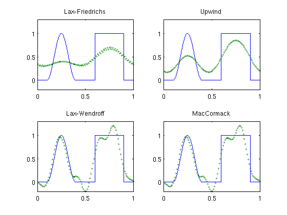
I have found a good test case from Matlab (squared cosine function and a double step function (my test only takes the more difficult latter) showing how FD methods behave. What we see here is Lax-Friedrichs is
diffusive. The 2nd order methods preserve smooth profile but introduce
spurious o
scilllations around the 2 discontinuities. BTW the classic upwind scheme is less diffusive than LF.
Coming up (my input)
1. Roberts-Weiss, Lax-Friedrichs and Duffy modified upwind (in Anchor article) for our current Pde (call it TEST CASE 2). double step function
2. Ditto for squared cosine function.
Re: About solving a transport equation
Posted: February 12th, 2020, 5:23 pm
by Cuchulainn
Matlab example
Re: About solving a transport equation
Posted: February 12th, 2020, 6:05 pm
by Cuchulainn
Re: About solving a transport equation
Posted: February 12th, 2020, 6:05 pm
by Cuchulainn
Re: About solving a transport equation
Posted: February 12th, 2020, 6:07 pm
by Cuchulainn
Roberts Weiss is centred in space...

Re: About solving a transport equation
Posted: February 12th, 2020, 6:13 pm
by Paul
1) You like transforming coords. So change to coords that move with the chars.
Or
2) Constrain dy and dt so that you solve numerically along the chars. That’s what I’ve used in the past.
Re: About solving a transport equation
Posted: February 12th, 2020, 8:31 pm
by Cuchulainn
Test case 2 with [$]u(y,0) = -sin (3.1415*y)[$]
Lax Friedrichs preserves the sinusoid's shape very well but gives big amplitude errors.
X MOC exact solution X Lax - Friedrichs
- 1 - 0.047012512 - 1 9.26536E-05
- 0.95 0.109823181 - 0.95 0.062928934
- 0.9 0.263954822 - 0.9 0.127034635
- 0.85 0.411587402 - 0.85 0.190821631
- 0.8 0.54908593 - 0.8 0.252637116
- 0.75 0.673064937 - 0.75 0.310813037
- 0.7 0.780471826 - 0.7 0.363718603
- 0.65 0.86866204 - 0.65 0.409813781
- 0.6 0.935464171 - 0.6 0.44770155
- 0.55 0.979233425 - 0.55 0.476176632
- 0.5 0.998892122 - 0.5 0.494268532
- 0.45 0.993956227 - 0.45 0.50127699
- 0.4 0.964547271 - 0.4 0.496798324
- 0.35 0.911389359 - 0.35 0.480741656
- 0.3 0.835791337 - 0.3 0.453334553
- 0.25 0.73961457 - 0.25 0.415118163
- 0.2 0.62522711 - 0.2 0.366932416
- 0.15 0.495445389 - 0.15 0.309892311
- 0.1 0.353464876 - 0.1 0.245356538
- 0.05 0.202781398 - 0.05 0.174889893
3.19189E-16 0.047105062 3.19189E-16 0.100220988
0.05 - 0.109731088 0.05 0.023196677
Re: About solving a transport equation
Posted: February 12th, 2020, 8:41 pm
by Cuchulainn
Test case 2 with [$]u(y,0) = - sin(pi*y)[$]
DD's upwinding preserves the sinusoid's shape very well and gives small amplitude errors, e.g. NY = 40, NT = 30 gives an error of 0.04.
X MOC exact solution X DD upwinding
- 1 - 0.047012512 - 1 9.26536E-05
- 0.95 0.109823181 - 0.95 0.116150727
- 0.9 0.263954822 - 0.9 0.264166963
- 0.85 0.411587402 - 0.85 0.410727521
- 0.8 0.54908593 - 0.8 0.547646404
- 0.75 0.673064937 - 0.75 0.671113014
- 0.7 0.780471826 - 0.7 0.778057221
- 0.65 0.86866204 - 0.65 0.865844274
- 0.6 0.935464171 - 0.6 0.932312625
- 0.55 0.979233425 - 0.55 0.975825696
- 0.5 0.998892122 - 0.5 0.995312114
- 0.45 0.993956227 - 0.45 0.990292087
- 0.4 0.964547271 - 0.4 0.960889218
- 0.35 0.911389359 - 0.35 0.90782746
- 0.3 0.835791337 - 0.3 0.832413292
- 0.25 0.73961457 - 0.25 0.736503554
- 0.2 0.62522711 - 0.2 0.622459721
- 0.15 0.495445389 - 0.15 0.493089766
- 0.1 0.353464876 - 0.1 0.351579019
- 0.05 0.202781398 - 0.05 0.20141174
3.19189E-16 0.047105062 3.19189E-16 0.046285327
0.05 - 0.109731088 0.05 - 0.109980717
0.1 - 0.263865454 0.1 - 0.263538831
0.15 - 0.411502959 0.15 - 0.410608125

